Introduction
Rendering in R
The rendering by rgl within R is done using OpenGL 1.x
(OGL1) code written largely by Daniel Adler in C++. OGL1 versions were
released in the late 1990s, and rgl in the early 2000s.
It’s unlikely that this will ever be updated to a more modern system:
I’d prefer to move away from doing any rendering at all, and leave that
to browsers that can display WebGL.
Rendering by rgl in web pages is done using WebGL 1 in
Javascript code written by me. This is likely to be updated in the
future, but for now the goal is to keep things simple, so compatibility
with OGL1 is needed. I wrote code to generate shaders that automatically
interpret things similar to the way OGL1 does it. There are facilities
to support user-defined shaders, and they could use much more modern
code; it’s also possible that the whole Javascript system will be
updated to use a modern Javascript library rather than working with
WebGL 1 forever.
Rendering assumed by glTF
The glTF 2.0 format is much newer, with its first release in 2017. It
assumes shaders are available that can interpret parameters described in
terms of physically based rendering (PBR). This is a much more realistic
system than OGL1 rendering. It aims for photo-realism, rather than the
diagram-style rendering targeted by rgl.
What is this document about?
The rgl2gltf package is intended to allow
rgl scenes to be saved to files using glTF 2.0 formats,
i.e. .gltf or .glb files, and objects from
those files to be incorporated into rgl displays. Since
those files assume PBR, we need to work out how to approximate the PBR
appearance in OGL1 rendering and vice versa.
Detailed calculations
OGL1 rendering in rgl
The appearance of objects in rgl is controlled by some
of the properties controlled by rgl::material3d(). These
are the default settings:
library(rgl)
material3d()
#> $color
#> [1] "#000000"
#>
#> $alpha
#> [1] 1
#>
#> $lit
#> [1] TRUE
#>
#> $ambient
#> [1] "#000000"
#>
#> $specular
#> [1] "#FFFFFF"
#>
#> $emission
#> [1] "#000000"
#>
#> $shininess
#> [1] 50
#>
#> $smooth
#> [1] TRUE
#>
#> $front
#> [1] "filled"
#>
#> $back
#> [1] "filled"
#>
#> $size
#> [1] 3
#>
#> $lwd
#> [1] 1
#>
#> $fog
#> [1] TRUE
#>
#> $point_antialias
#> [1] FALSE
#>
#> $line_antialias
#> [1] FALSE
#>
#> $texture
#> NULL
#>
#> $textype
#> [1] "rgb"
#>
#> $texmipmap
#> [1] FALSE
#>
#> $texminfilter
#> [1] "linear"
#>
#> $texmagfilter
#> [1] "linear"
#>
#> $texenvmap
#> [1] FALSE
#>
#> $depth_mask
#> [1] TRUE
#>
#> $depth_test
#> [1] "less"
#>
#> $isTransparent
#> [1] FALSE
#>
#> $polygon_offset
#> [1] 0 0
#>
#> $margin
#> [1] ""
#>
#> $floating
#> [1] FALSE
#>
#> $tag
#> [1] ""
Colors are assumed to be RGB with 8 bits per channel defined using R
color notation, for example "#FF0000" is pure red.
alpha controls transparency, running from 0 to 1: 0 is
fully transparent (invisible), 1 is fully opaque. If lit is
FALSE, that’s it: the color is displayed without any
modification.
When lit = TRUE the shading algorithm comes into play.
The material properties ambient, specular and
emission are additional colors, and the
shininess, smooth and fog
parameters come into the calculation. There’s a possibility to have a
single texture: an image file whose characteristics can be
used to modify the color or alpha channel, with a location in the image
defined by “texture coordinates” associated with the surface being
rendered.
The above parameters are combined with global properties of the
lighting: it has a direction as well as ambient,
diffuse and specular colors.
Consider the following image:
xyz <- cbind(c(0, 1, 1, 0), c(0, 0, 1, 1), c(0, 0, 1, 1))
st <- xyz[, 1:2]
quads3d(xyz,
        texcoords = st,
        texture = system.file("textures/rgl2.png", package = "rgl"),
        color = "steelblue")
This is drawn using these two automatically generated shaders. The vertex shader controls the positioning of the quadrilateral. It is called for each vertex of the quad, and controls the position where they are displayed.
  /* ****** quads object 13 vertex shader ****** */
#ifdef GL_ES
#ifdef GL_FRAGMENT_PRECISION_HIGH
  precision highp float;
#else
  precision mediump float;
#endif
#endif

  /* these are constants for all vertices */
  uniform mat4 mvMatrix;
  uniform mat4 prMatrix;
  uniform mat4 normMatrix;

  /* these are properties associated with each vertex */
  attribute vec3 aPos;
  attribute vec4 aCol;
  attribute vec3 aNorm;
  attribute vec2 aTexcoord;

  /* These are computed and passed to the fragment shader */
  varying vec4 vCol;
  varying vec4 vPosition;
  varying vec4 vNormal;
  varying vec2 vTexcoord;

  void main(void) {
    vPosition = mvMatrix * vec4(aPos, 1.);
    gl_Position = prMatrix * vPosition;
    vCol = aCol;
    vNormal = normMatrix * vec4(-aNorm, dot(aNorm, aPos));
    vTexcoord = aTexcoord;
  }
The fragment shader is called for each pixel on the surface of the quad, and controls the appearance. I’ve improved the formatting a bit and added extra comments:
/* ****** quads object 13 fragment shader ****** */
#ifdef GL_ES
#ifdef GL_FRAGMENT_PRECISION_HIGH
  precision highp float;
#else
  precision mediump float;
#endif
#endif

  /* these variables are interpolated
     between the values calculated for each vertex */

  varying vec4 vCol; // carries alpha
  varying vec4 vPosition;
  varying vec2 vTexcoord;
  varying vec4 vNormal;

  /* these are constant for all fragments */
  uniform sampler2D uSampler;
  uniform int uFogMode;
  uniform vec3 uFogColor;
  uniform vec4 uFogParms;
  uniform mat4 mvMatrix;
  uniform vec3 emission;
  uniform float shininess;
  uniform vec3 ambient0;
  uniform vec3 specular0; // light*material
  uniform vec3 diffuse0;
  uniform vec3 lightDir0;
  uniform bool viewpoint0;
  uniform bool finite0;

  void main(void) {

    /* these are local variables */

    vec4 fragColor;
    vec3 n = normalize(vNormal.xyz);
    vec3 eye = normalize(-vPosition.xyz);
    vec3 lightdir;
    vec4 colDiff;
    vec3 halfVec;
    vec4 lighteffect = vec4(emission, 0.);
    vec3 col;
    float nDotL;

    n = -faceforward(n, n, eye);
    colDiff = vec4(vCol.rgb * diffuse0, vCol.a);
    lightdir = lightDir0;
    if (!viewpoint0)
      lightdir = (mvMatrix * vec4(lightdir, 1.)).xyz;
    if (!finite0) {
      halfVec = normalize(lightdir + eye);
    } else {
      lightdir = normalize(lightdir - vPosition.xyz);
      halfVec = normalize(lightdir + eye);
    }
    col = ambient0;
    nDotL = dot(n, lightdir);
    col = col + max(nDotL, 0.) * colDiff.rgb;
    col = col + pow(max(dot(halfVec, n), 0.), shininess) * specular0;
    lighteffect = lighteffect + vec4(col, colDiff.a);
    vec4 textureColor = lighteffect*vec4(texture2D(uSampler, vTexcoord).rgb, 1.);
    fragColor = textureColor;
    float fogF;
    if (uFogMode > 0) {
      fogF = (uFogParms.y - vPosition.z/vPosition.w)/(uFogParms.y - uFogParms.x);
      if (uFogMode > 1)
        fogF = mix(uFogParms.w, 1.0, fogF);
      fogF = fogF*uFogParms.z;
      if (uFogMode == 2)
        fogF = 1.0 - exp(-fogF);
      else if (uFogMode == 3)
        fogF = 1.0 - exp(-fogF*fogF);
      fogF = clamp(fogF, 0.0, 1.0);
      gl_FragColor = vec4(mix(fragColor.rgb, uFogColor, fogF), fragColor.a);
    } else gl_FragColor = fragColor;
  }
I’ll use the same notation as https://www.khronos.org/registry/glTF/specs/2.0/glTF-2.0.html#implementation, plus some more:
- \(V\) is the normalized vector from the shading location to the eye
- \(L\) is the normalized vector from the shading location to the light
- \(N\) is the surface normal in the same space as the above values
- \(H\) is the half vector, where \(H = normalize(L + V)\)
-
\(\chi^+(x)\) is the Heaviside
function
max(x, 0) -
\(s\) is the
shininess - \(C_a\), \(C_d\), \(C_s\) and \(C_e\) are the material colors, ambient, diffuse (just color in the material), specular and emission respectively.
- \(L_a\), \(L_d\) and \(L_s\) are the ambient, diffuse and specular light values respectively.
Ignoring fog and texture for now, the fragment shader implements the
following computation of the color at a particular location: \[
C_e + C_aL_a + \chi^+(N \cdot L) C_d L_d + \chi^+(H \cdot N)^s C_sL_s
\] The texture multiplies this value by the texture color at that
location, and fog mixes it with the fog color in a proportion determined
by the fogMode parameter and the depth in the scene.
PBR rendering in glTF
The glTF specification presents a sample implementation, with several comments following to describe possible improvements. The simple computation introduces some new notation based on the material properties in glTF:
-
\(\alpha\) is the square of the
roughnessvalue -
\(m\) is the
metallicvalue between 0 and 1 - \(\textit{lerp}(a, b, t)\) is the linear interpolation function returning \((1-t)a + tb\), aka \(\textit{mix}(a, b, t)\).
Using this notation and the previous notation, it computes the
“bidirectional reflectance distribution function” or BRDF as \[
D(\alpha) := \frac{1}{\pi}\frac{\alpha^2 \chi^+(N \cdot H)}{[(N \cdot
H)^2 (\alpha^2 - 1) + 1]^2} \\
G(\alpha) := \frac{2 | N \cdot L | \chi^+(H \cdot L)}{|N\cdot L| +
\sqrt{\alpha^2 + (1-\alpha^2)(N \cdot L)^2}}\frac{2|N\cdot V|\chi^+(H
\cdot V)}{|N \cdot V| + \sqrt{\alpha^2 + (1-\alpha^2)(N \cdot V)^2}}\\
\textit{f0} \leftarrow \textit{lerp}(0.04, C_d, m) = 0.04(1-m) + mC_d \\
F \leftarrow \textit{f0} + (1 - \textit{f0})(1- |V \cdot H|)^5
\\
\textit{f_diffuse} \leftarrow \frac{1}{\pi}(1-F)\textit{lerp}(C_d, 0, m)
= \frac{1}{\pi}(1-F)(1-m)C_d\\
\textit{f_specular} \leftarrow \frac{F D(\alpha) G(\alpha)}{4 |V\cdot N|
|L \cdot N|}
\] These values are combined into a single value
f_diffuse + f_specular which is multiplied by cosine of the
incoming light angle (\(N \cdot L\) in
the notation above) and used in ray-tracing based rendering.
Assumptions in the approximations
The default light in rgl has all of \(L_a\), \(L_d\) and \(L_s\) being white, i.e. 1. Most materials
have \(C_a\) and \(C_e\) set to black, i.e. 0. We can thus
ignore ambient and emission contributions, or assume they add to the
diffuse and specular contributions from the formula. With that
assumption, the output from rgl simplifies to \[
\chi^+(N \cdot L) C_d + \chi^+(H \cdot N)^s C_s
\]
We’ll also assume that \(C_d\) is
fixed as color in rgl and as
baseColor in PBR. Then matching given PBR parameters in
OGL1 terms comes down to using them to choose shininess \(s\) and specular color \(C_s\) so that the expression above, which
defines a function depending on \(N\),
\(L\) and \(V\), approximates the BRDF calculation
which defines a different function depending on those three vectors.
We start by rotating the coordinate system so that \(N = (0,0,1)\) and \(V = (\sin \theta, 0, \cos \theta)\), where \(\theta\) is the angle between \(V\) and \(N\), and \(V \cdot N = \cos \theta\).
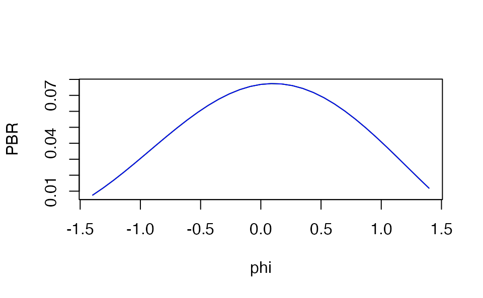
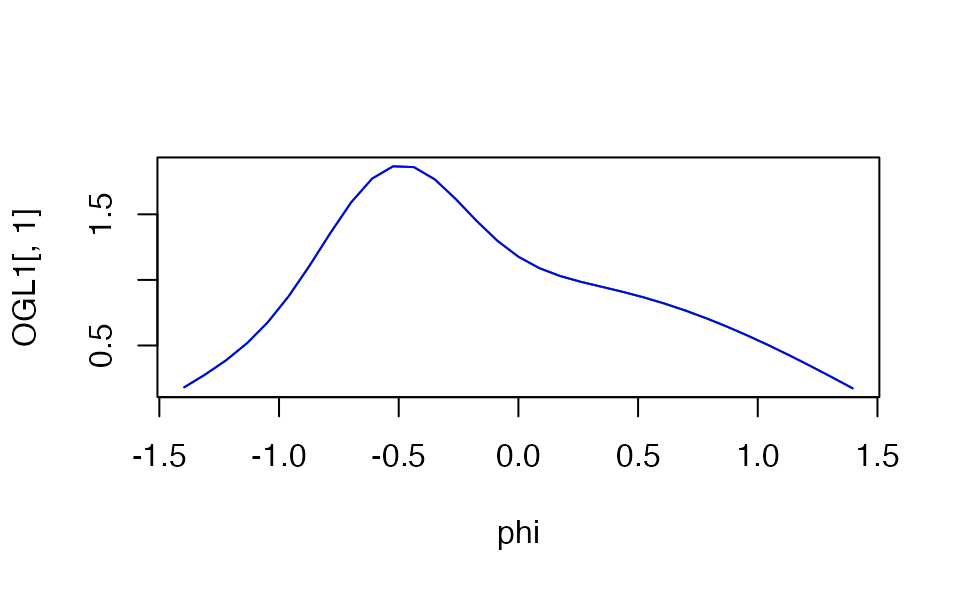
What we’d like to do is to match the appearance over the whole range of \(\theta\) and \(L\), but that seems hard, so instead we’ll try a few fixed values of \(\theta\) and try to match graphs of BRDF and OGL1.
Let’s try it:
# Typical PRB parameters
roughness <- 1
metalness <- 1
baseColor <- c(1, 1, 1)

# Default rgl parameters
s <- 50
Cs <- c(1,1,1)

Cd <- baseColor
m <- metalness
alpha <- roughness^2

h <- c(0.999, 0.5)

N <- c(0,0,1)
theta <- 30 * pi/180 # angle between V and N
V <- c(sin(theta), 0, cos(theta))
VdotN <- sum(V*N)


phi <- seq(-80, 80, by = 5)*pi/180 # angle between L and N
PBR <- OGL1 <- matrix(NA, nrow=length(phi), ncol=3)
for (j in seq_along(phi)) {
  L <- c(sin(phi[j]), 0, cos(phi[j]))
  H <- (L + V)/sqrt(sum((L + V)^2))
  HdotN <- sum(H*N)
  HdotL <- sum(H*L)
  NdotL <- sum(N*L)
  HdotV <- sum(H*V)
  D <- (1/pi)*alpha^2*max(0, HdotN)/(HdotN^2 * (alpha^2 - 1) + 1)^2
  G <- 2*NdotL*max(HdotL, 0)*2*VdotN*max(HdotV, 0)/
    (NdotL + sqrt(alpha^2+ (1-alpha^2)*NdotL^2))/
    (VdotN + sqrt(alpha^2+ (1-alpha^2)*VdotN^2))
  f0 <- 0.04*(1-m) + m*Cd
  F <- f0 + (1 - f0)*(1 - HdotV)^5
  f_diffuse <- (1/pi)*(1-F)*(1-m)*Cd
  f_specular <- F*D*G/4/abs(VdotN)/abs(NdotL)
  PBR[j,] <- (f_diffuse + f_specular)*NdotL
  OGL1[j,] <- max(NdotL, 0)*Cd + max(HdotN, 0)^s*Cs
}
plot(phi, PBR[,1], type="l", col = "red", ylim=range(PBR), ylab="PBR")
lines(phi, PBR[,2], col = "green")
lines(phi, PBR[,3], col = "blue")
plot(phi, OGL1[,1], type="l", col = "red", ylim=range(OGL1))
lines(phi, OGL1[,2], col = "green")
lines(phi, OGL1[,3], col = "blue")
This looks pretty hopeless.